采用MATLAB对正弦信号，语音信号进行生成、采样和内插恢复，利用MATLAB工具箱对混杂噪声的音频信号进行滤波

一、正弦信号的采样与重建

要求：固定采样频率500 kHz，分别对100 kHz、250 kHz、400 kHz的正弦波信号（幅度，相位自定义）进行采样和重建，分析比较原信号与重建信号的波形。
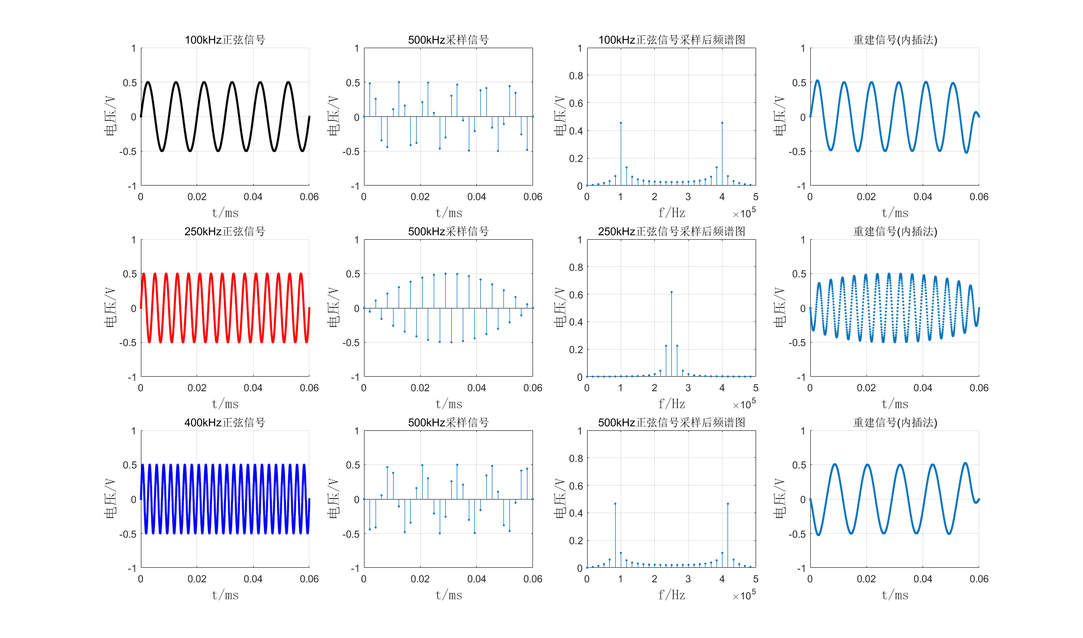
最终整体结果如下图：

1、正弦信号的生成：

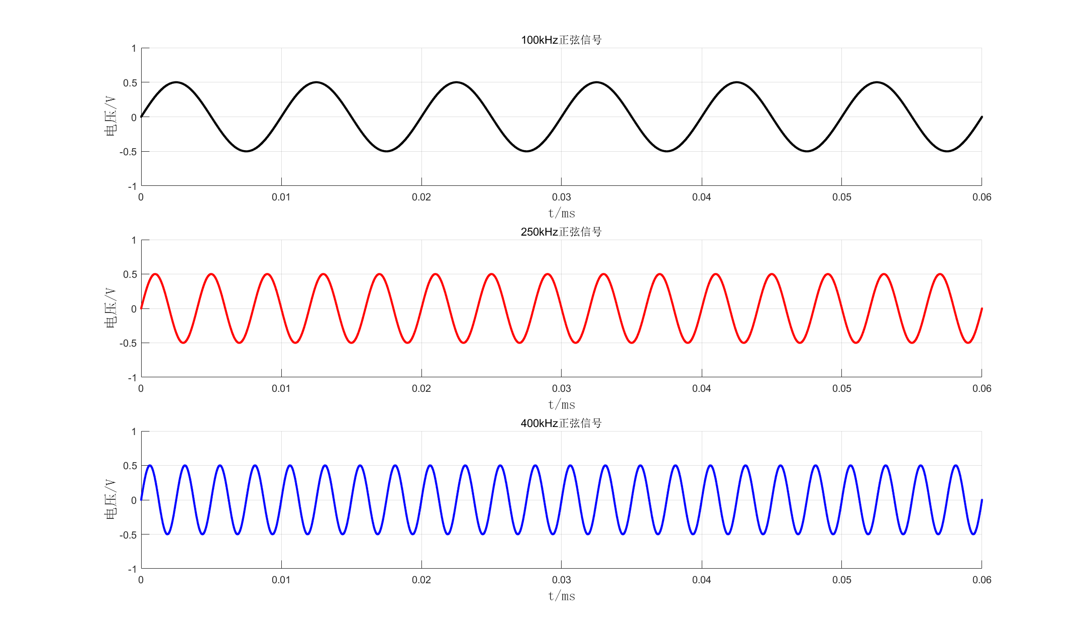
三个正弦信号的生成如下图所示：

①代码实现：

  因为被采样信号频率为100,250和400kHz，因此选取时间窗时间范围tscale为6e-5s，并选取采样点数为10000。通过密集点数来对模拟信号进行模拟生成。为了实验方便，取三个信号初始相位均为0，幅度为0.5V。在MATLAB画图时采用了画散点图函数scatter，为了在后续信号恢复时能更清晰地看出点的恢复。

2、正弦信号的采样（点图及频谱图）：

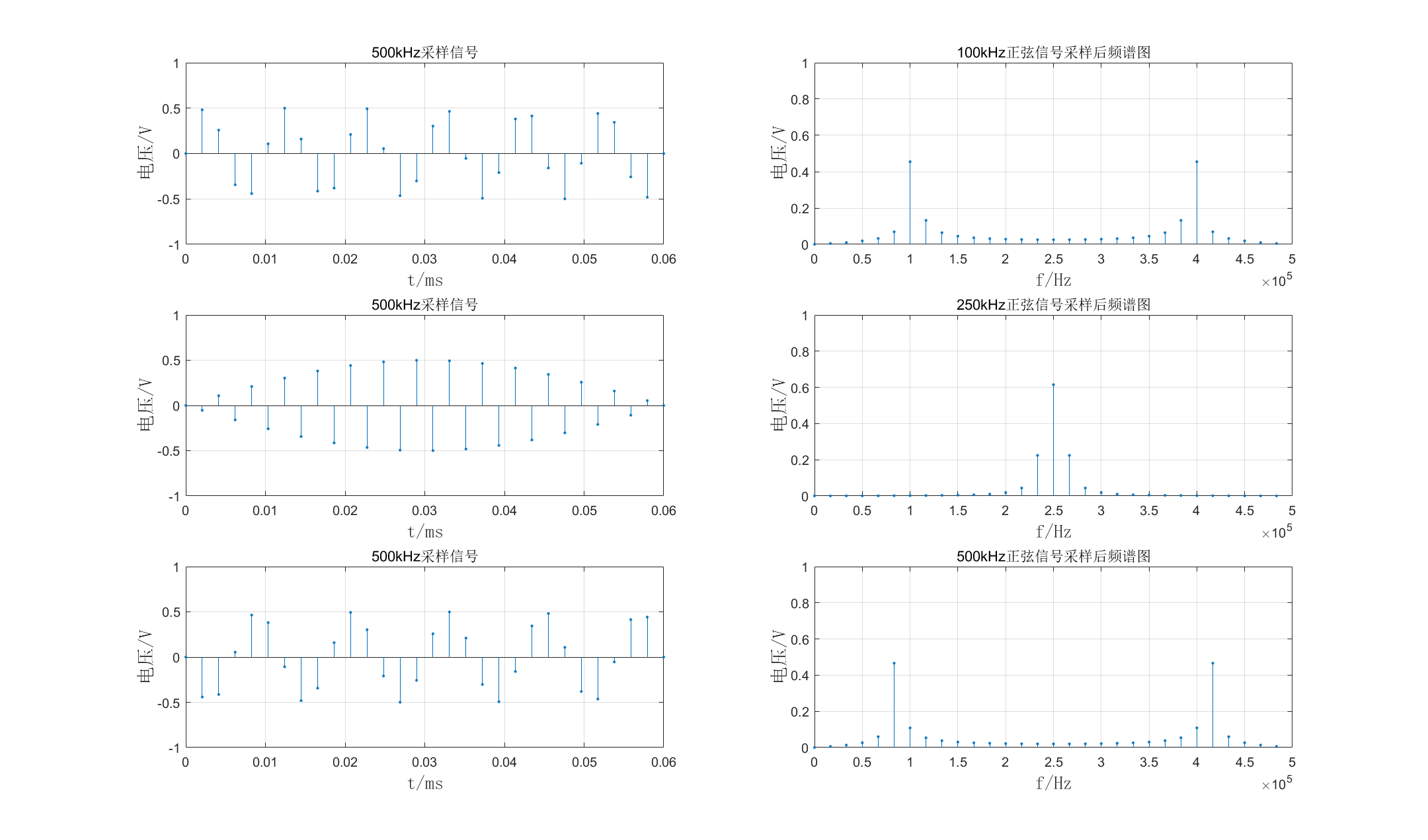
三个正弦信号的采样结果如下图所示，左侧三个图为采样后波形，右侧三个图为采样信号的频谱图：

①代码实现：

  由时间窗范围tscale和采样频率f为500kHz可得三个信号的采样点数为30个，因此在0到tscale之间建立采样点数n_point为30的时间序列t，对三个信号进行重新生成，即如以下代码所示：

% ==========画采样后的图========== %
k = 1;
n_point = (k * tscale) / (1 / 500000);

t = linspace(0, k * tscale, n_point);
Y1 = A * sin(2 * pi * f1 * t);  % 0.5为振幅。

其中k为时间窗倍率，如果想多采样点数进行频谱生成则增大k值。f1为100kHz频率。矩阵Y1为在t时间间隔矩阵下新生成的函数，也可看作为在f为500kHz下的采样100kHz的函数。250和400kHz的函数采样同上述方法。
  频谱的生成采用fft函数，输入采样信号矩阵Y1并输出同维矩阵yf1，但此时的yf1并不能直接表示信号的频率，只能表示频率间的相对关系，通过以下变换得到对应频谱函数中的横纵坐标：

% ==========画采样后的频谱图========== %
fs = 500000;

yf1 = fft(Y1);
subplot(3, 2, 2);
realy = 2 * abs(yf1(1 : n_point)) / n_point;
realf = (0 : n_point - 1) * (fs / n_point);   

其中realf为变换后得到的频谱函数横坐标序列，realy为变换后得到的频谱函数幅值的序列。其中realf采用归一法，将0到n_point-1共n_point个点除以n_point，将频率的n_point个点全部锁定在0到1范围之间，然后乘以最高的采样频率fs即可将相互之间具有一定关系对的点分不到0到fs之间，从而构成了具有物理意义频谱序列。250和400kHz的函数频谱图生成同上述方法。

②结果分析：

  100kHz采样信号的频谱在100kHz和400kHz处有较大值，其中100kHz为原始正弦信号频率，400kHz为信号频谱负数频率中的-100kHz经过500kHz信号频率向右搬移得到，原理如下图所示(不小心画了个诡异的笑脸)：
[外链图片转存失败,源站可能有防盗链机制,建议将图片保存下来直接上传
  250kHz采样信号的频谱原理同上，因为信号原频率和搬移后频率重合，因此其幅度值大于0.5。
  500kHz采样信号不满足采样定理，发生频谱混叠，但是因为采样信号只有一个主要频率，因此不明显。

3、正弦信号的恢复（内插法重建）：

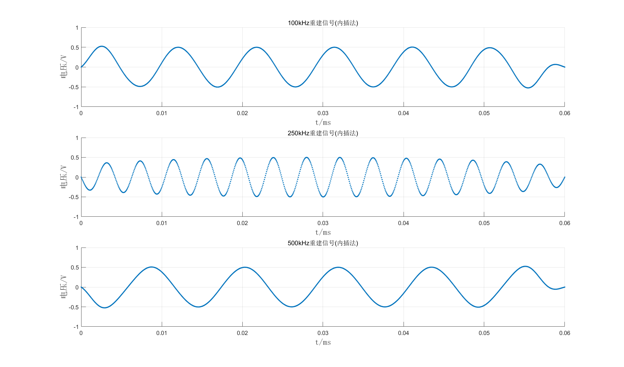
三个正弦信号的恢复结果如下图所示：

①代码实现：

  采用内插法实现信号恢复（重建），内插法的数学公式如下所示：
$$\begin{gathered} y(t)=x_a(t)={\int }_{-\infty }^{\infty }{\hat{x}}_a(ı)h(t-ı)dı \\ =\sum _{n=-\infty }^{\infty }{x}_a(nT)\frac{\sin [\frac{\pi }{T}(t-nT)]}{\frac{\pi }{T}(t-nT)} \end{gathered}$$
  对以上数学公式进行MATLAB代码实现为：

% ==========恢复波形========== %
%原理(内插法): y(t)=Σx(n)*sinc((t-nTs)/Ts)
n_point = (k * tscale) / (1 / 500000);  % 采样点数
ts = 1 / fs;  % 采样时间间隔
to = linspace(0, k * tscale, n_point);
K = 30;  % 还原后的信号点倍数
dt = ts / K;  % 还原后的点时间间隔
ta = 0 : dt : n_point * ts;

figure;
% =====信号1===== %
y_recover1 = zeros(length(ta), 1);  % 恢复信号y，先建立一个0矩阵，从0到1，时间间隔为dt
for t = 0 : length(ta) - 1  % 求过采样后的每个值
	for m = 0 : length(to) - 1  % 累加sinc与原函数对应点的积
		y_recover1(t + 1) = y_recover1(t + 1) + Y1(m + 1) * sinc((t * dt - m * ts) / ts);
	end
end

其中外循环为求得恢复信号的序列的幅度值，内循环为对内插函数中原信号和抽样信号相乘的累加操作。t序列即为恢复信号中的时间序列t，m序列为原500kHz采样的周期序列，ts为500kHz采样信号的时间间隔（即对应内插公式中的大写周期T），dt为恢复信号的时间间隔。用ts除以K得到dt意思为恢复信号的点之间的间隔要比原采样信号的点时间间隔小30倍，即内插30个点。Y1为采样信号函数，对应公式中的$$x_a（nT）$$， y_recover为恢复信号函数。

②结果分析：

  经过抽样函数矩形框低通滤波器之后，100kHz的过采样信号被很好地还原，滤除了高频的400kHz；250kHz的临界采样信号，被还原的同时，通过整体来看，可以看出其每个波峰最高点连成的线又形成了一个新的低频正弦信号，这个在频谱图上是没有看到的，在和其他人交流时，发现均碰到这个问题，我感到很疑惑；400kHz的欠采样信号在经过低通滤波器后滤除了400kHz左右的信号，只保留了因频谱搬移得到的100kHz信号，但是其频率小于100kHz，被滤除的频率也略大于400kHz，这个问题我也仍没有解决。

二、语言信号的采样与重建

要求：采集一段音频信号，分别用欠采样、临界采样和过采样对信号进行重采样，并重建原音频信号，分析比较重建信号与原信号的差别。
最终整体结果如下图：

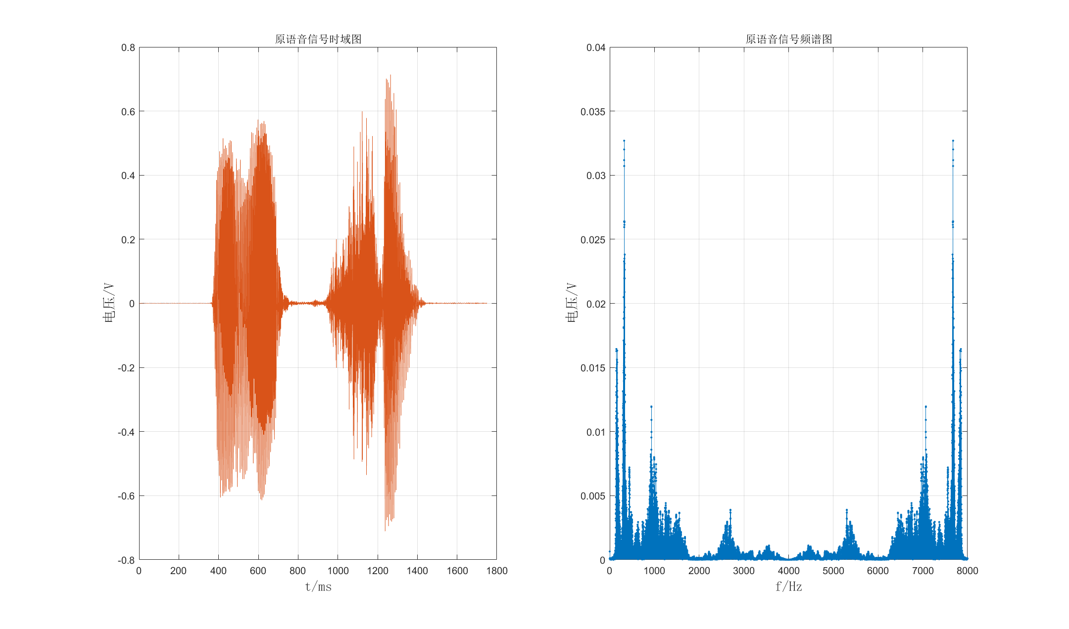
1、语音信号的生成：

语音信号的时域和频域图如下图所示：

①代码实现：

  通过audioread函数读取.wav语音信号文件。其他处理方式同前正弦信号。

②结果分析：

  由上图可见在0到8000Hz范围内，信号频谱关于4000Hz对称，且能量主要集中在1000Hz以下，因为人声信号的频率主要在0到600Hz。因此取窗范围为0到1000Hz，如下图所示：

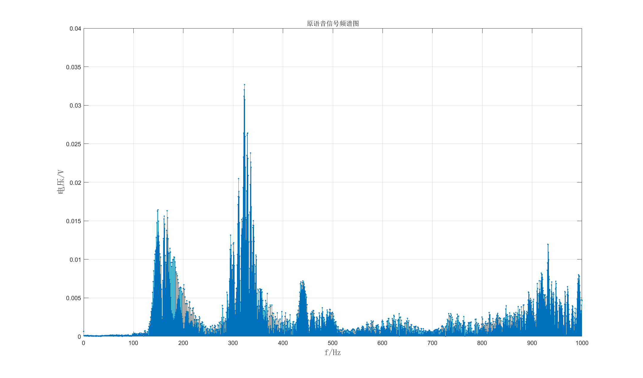
由图可见，信号频率能量的主要范围在300Hz左右，此范围为男中音。

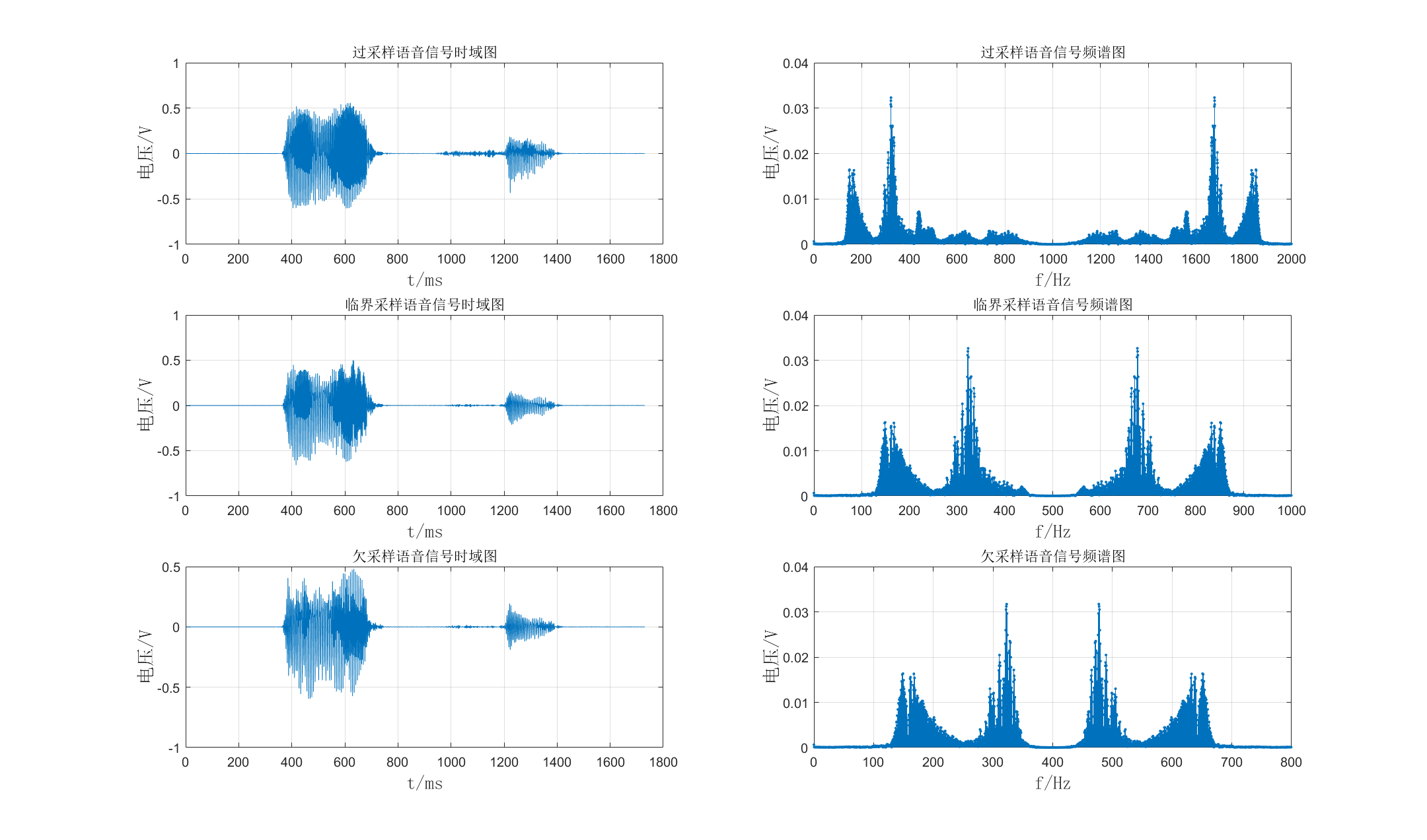
2、语音信号的采样：

由上图可知，设语音信号的频率主要在0到500Hz，因此设采样率为2000Hz时为过采样，1000Hz时为临界采样，800Hz时为欠采样。经过过采样，临界采样和欠采样后的时域和频域图如下图所示：

①代码实现：

  通过decimate函数减少采样倍率，在保持总时间不变的前提下减少采样点数。因此2000Hz，1000Hz和800Hz的减少倍率分别为4，8和10。相关代码如下所示：

% ==========减少采样率后的信号========== %
% 人的语音信号频率在0到600Hz之间，从原信号频谱可以看出信号能量在100到500Hz之间，因此以下取采样率为2000Hz为过采样，1000Hz为临界采样，800Hz为欠采样。
% =====过采样===== %
x1 = decimate(x, 4);
t1 = decimate(t, 4);
fs1 = fs / 4;
subplot(3, 2, 1);
plot(t1 .* 1000, x1);

分别要对时间序列和幅值序列进行倍减。

②结果分析：

  从时域角度看，曲线数目随采样率的减少而不断减少；从频域角度看，频谱在不断重叠。在欠采样信号中，混叠频率已经进入了声音的有效频率500Hz内，即发生了频谱的混叠。

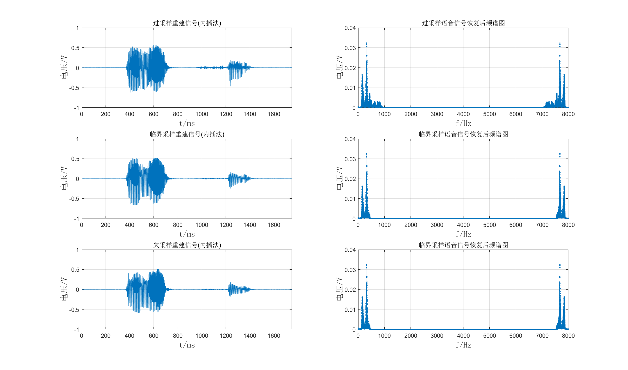
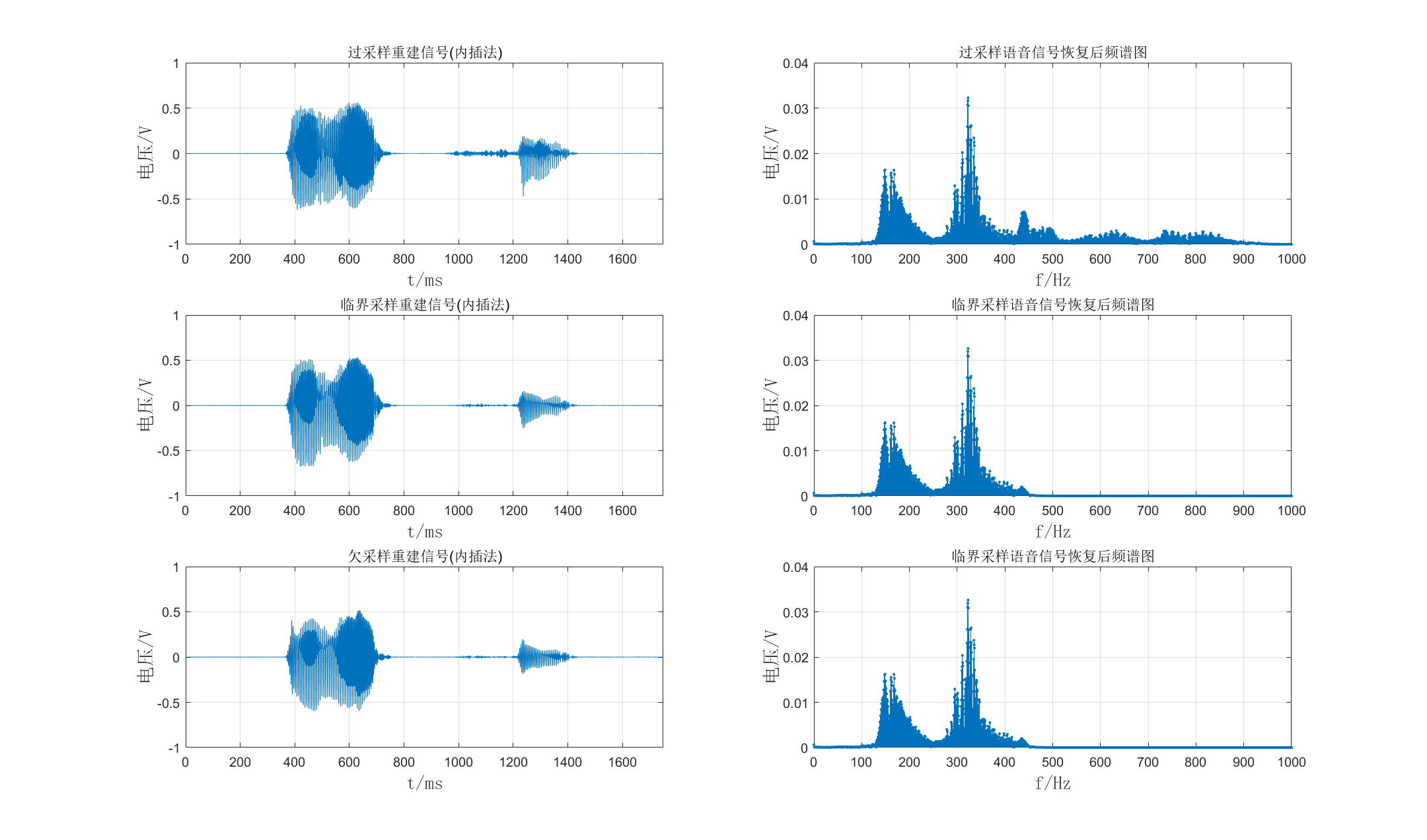
3、语音信号的恢复（内插法重建）：

三种采样信号的恢复结果如下图所示：

①代码实现：

  同样采用内插法实现信号恢复，原理方法和代码与正弦信号的相同，相关代码如下：

% ==========减少采样率后的信号恢复========== %
f = 8000;
f1 = 2000;
f2 = 1000;
f3 = 800;
tscale = 1;

% =====过采样===== %
n_point = 14000 / 4;  % 采样点数
ts = 1 / f1;  % 采样时间间隔
to = linspace(0, tscale, n_point);
K = 4;  % 还原后的信号点倍数
dt = ts / K;  % 还原后的点时间间隔
ta = 0 : dt : n_point * ts;
y_recover1 = zeros(length(ta), 1);  % 恢复信号y，先建立一个0矩阵，从0到1，时间间隔为dt

for t = 0 : length(ta) - 1  % 求过采样后的每个值
	for m = 0 : length(to) - 1  % 累加sinc与原函数对应点的积
		y_recover1(t + 1) = y_recover1(t + 1) + x1(m + 1) * sinc((t * dt - m * ts) / ts);
	end
end

相关变量的含义也与之前相同。

②结果分析：

  由上图中右侧的三幅信号恢复后的频谱图可知，临界采样和欠采样混叠部分的频率部分消失；左侧三幅恢复后的时域图与采样的时域图相比，曲线变得更密，但三幅图相互比较无很大区别。

三、小提琴音频的加噪去噪处理

要求：选择子作业１中的音频信号，自行给定滤波器的系统函数，分别采用时域线性卷积和差分方程两种方法对音频信号进行滤波处理，比较滤波前后信号的波形和回放的效果。
最终整体效果如下图：

1、音频信号的构建

①音乐信号的产生：

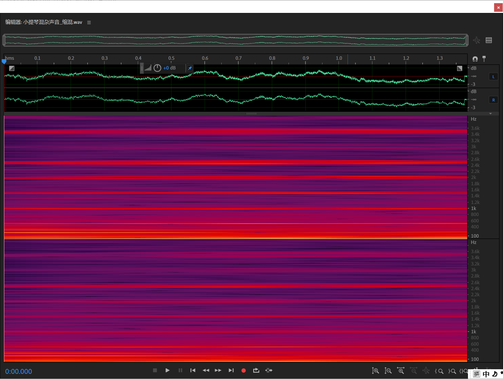
  采用Adobe Audition提取出一首小提琴音乐的一个音符的音频信号，如下图所示：

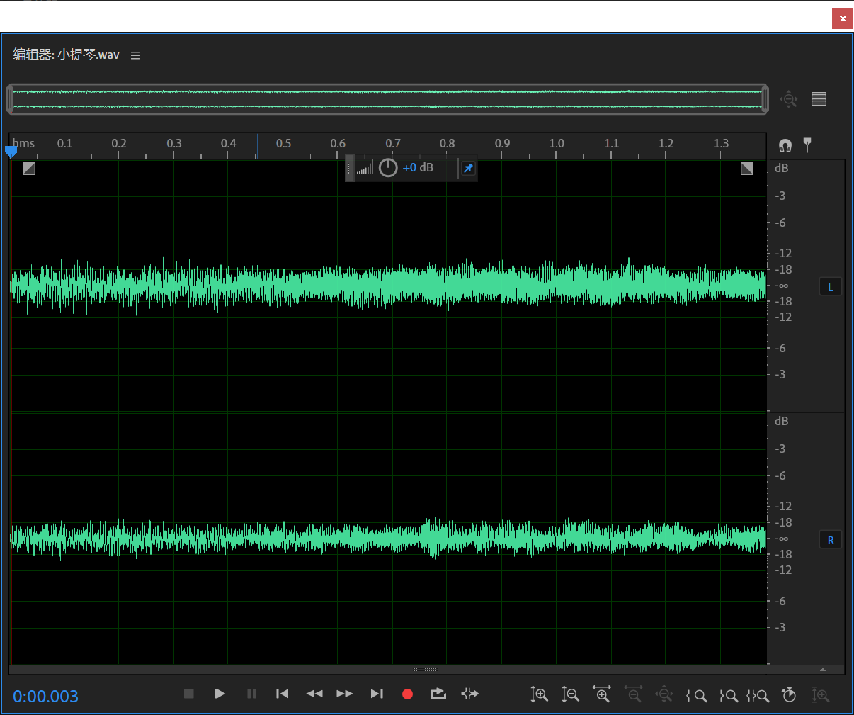
上下信号波形分别为左右声道。如何判断为一个音符的信号呢？通过Adobe Audition的频谱分析进行判断，语谱图如下图所示：

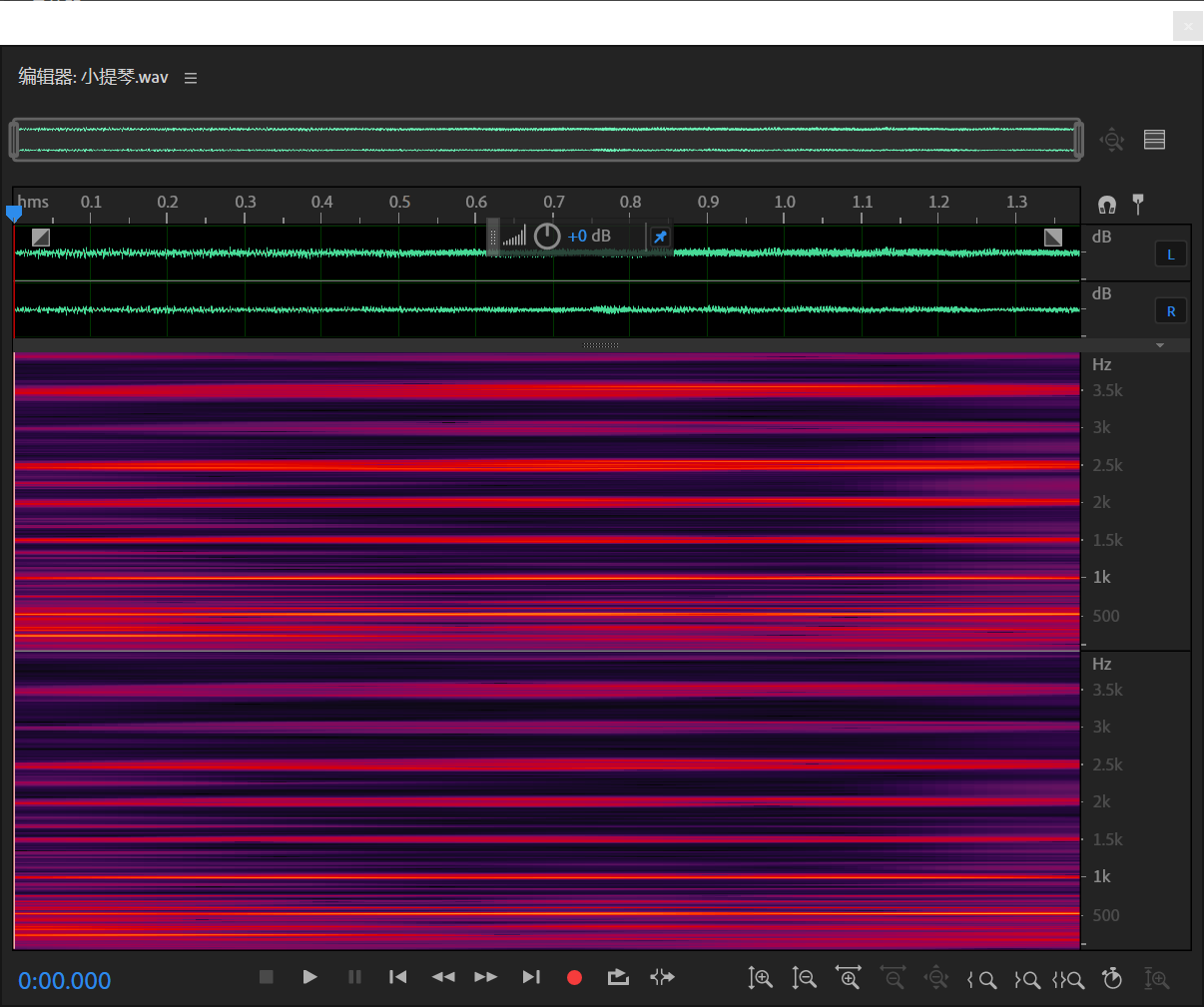
语谱图是将信号的频谱和时间结合，横轴为时间，纵轴为频率，颜色的深浅表征信号的幅度。通过在一段音乐信号的语谱图中，找到在一定时间段内各频率分量稳定的区间，则可判断其为一个音符。通过上图的各频率成分的颜色可得知，在该时间段下，在某几段频率区间中，颜色波形十分稳定。
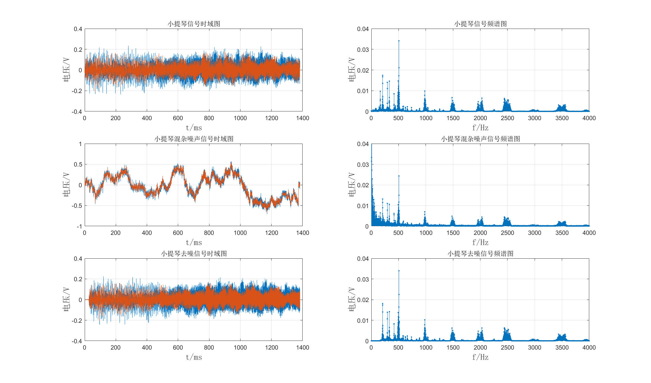
  通过MATLAB对该音乐信号进行频谱分析可得：（左图为时域信号，右图为频域信号）

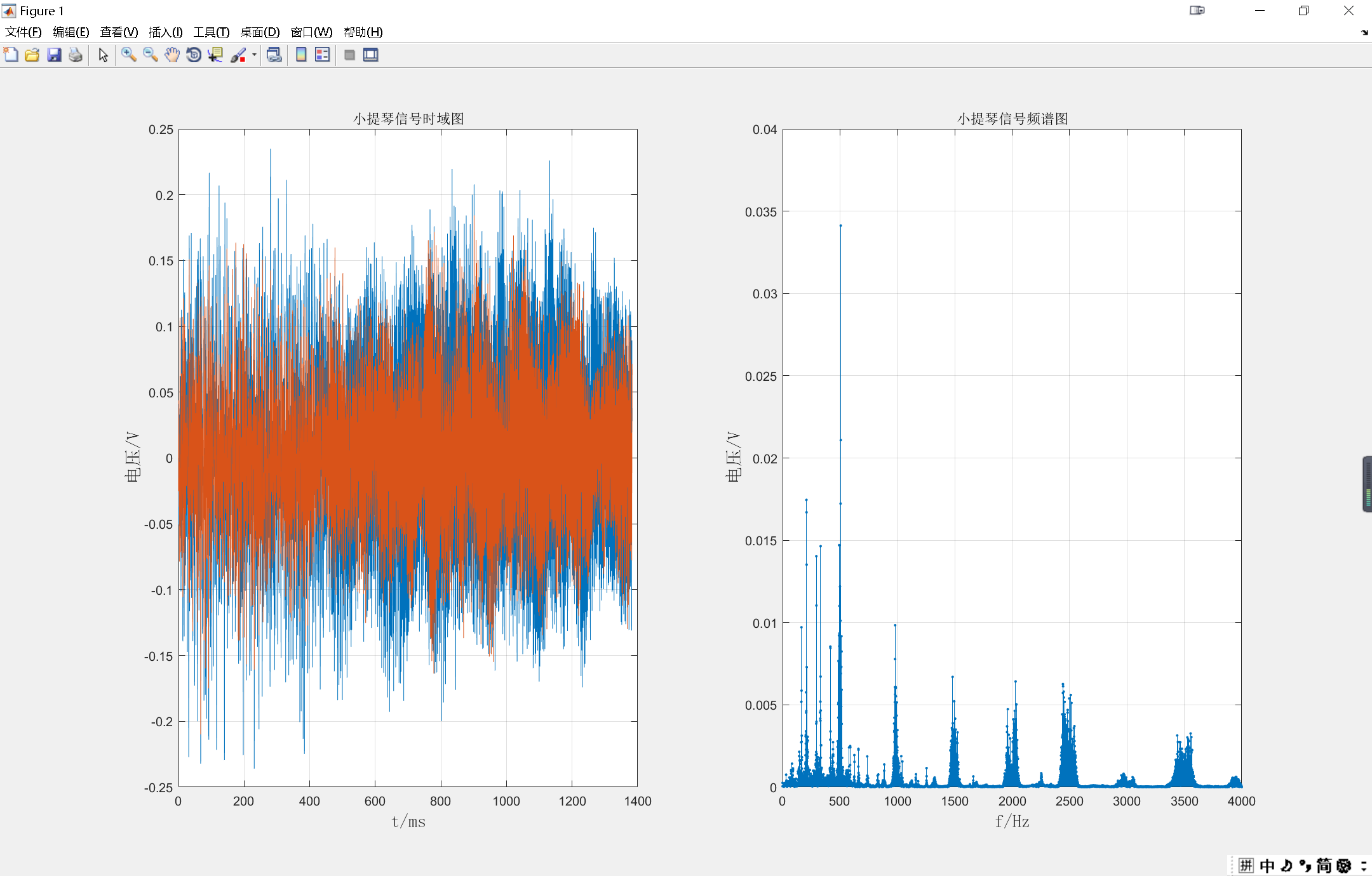
将上图与前一幅图对比可知，频域图显示能量高的地方，其对应语谱图上的颜色更鲜艳，则说明其表征了音频信号的能量分布。

②噪声信号的产生：

  因为本实验是要对信号作滤波处理，所以我在该音乐信号中通过Adobe Audition软件添加了主要能量分布在低频的高斯白噪声，其时域波形和语谱图如下图所示：

由上图可见，该噪声能量的大部分分布在400Hz以下，主要能量分布在100Hz以下，因此后续的滤波器设计选择使用低通滤波器。
  通过MATLAB对该噪声信号进行频谱分析可得：（左图为时域信号，右图为频域信号）

可见该噪声的主要能量分布在200Hz以下。

③混杂信号的产生：

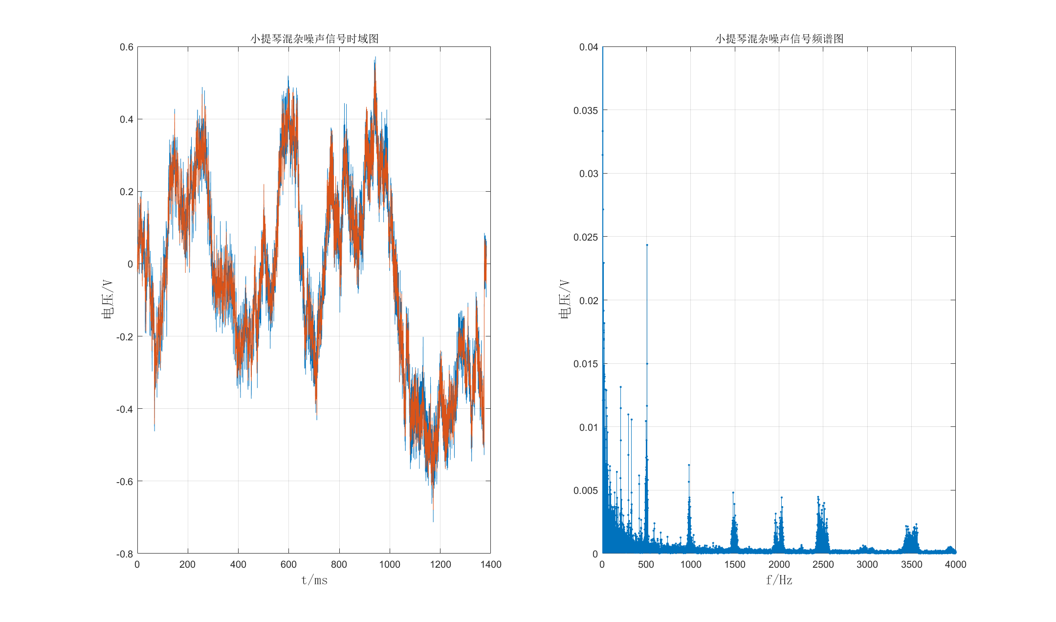
  通过Adobe Audition软件的多轨功能将音乐信号和噪声信号进行叠加，因此该噪声为加性噪声，叠加后的时域图和语谱图如下图所示：

由上图可知，在200Hz的频率成分以下叠加了主要的噪声。
  通过MATLAB对该混杂信号进行频谱分析可得：（左图为时域信号，右图为频域信号）

2、滤波器的设计

①MATLAB滤波器设计工具：

  在MATLAB的应用程序中选择Filter Design & Analysis如下图所示：

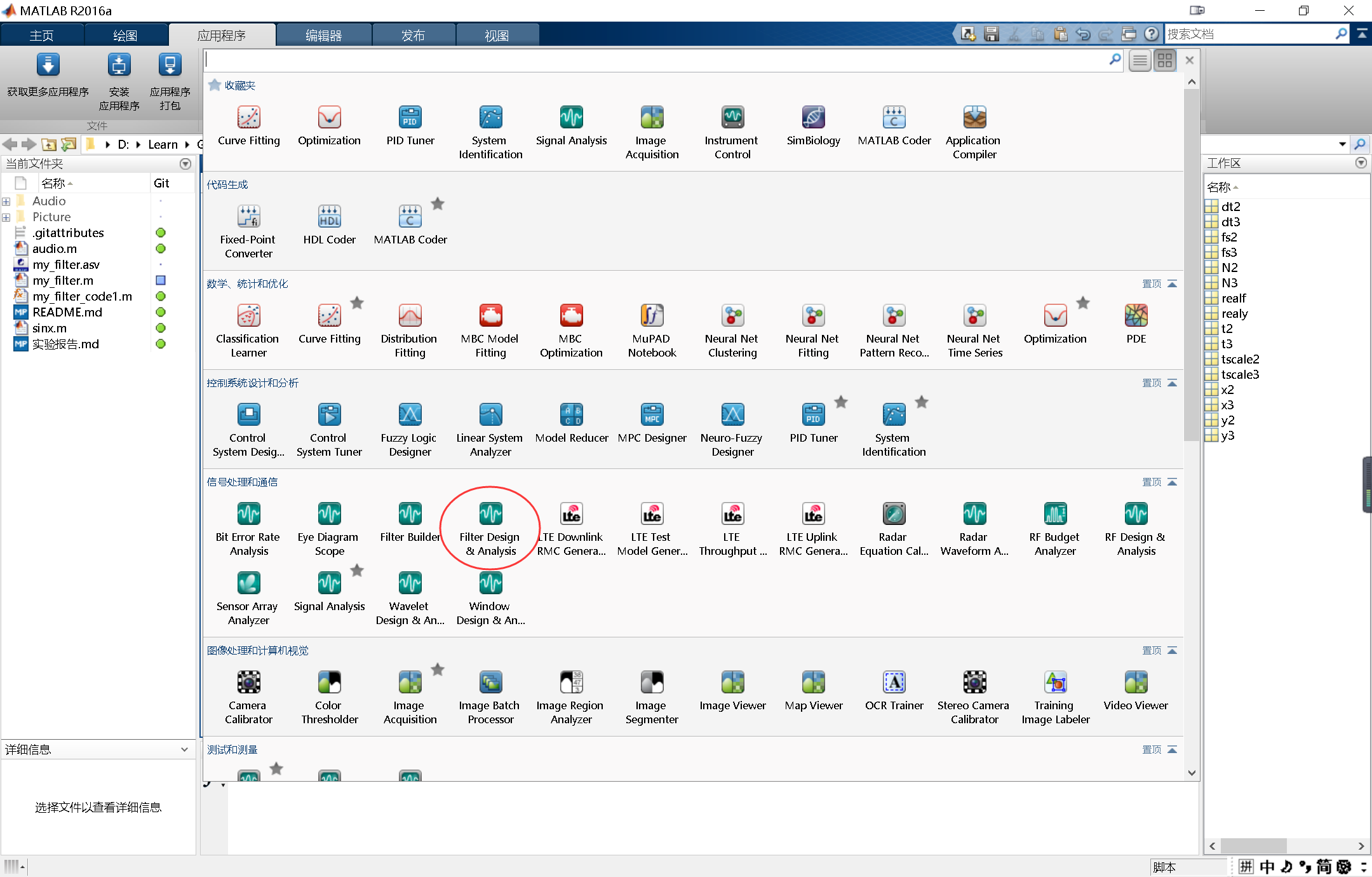
则得到如下界面：

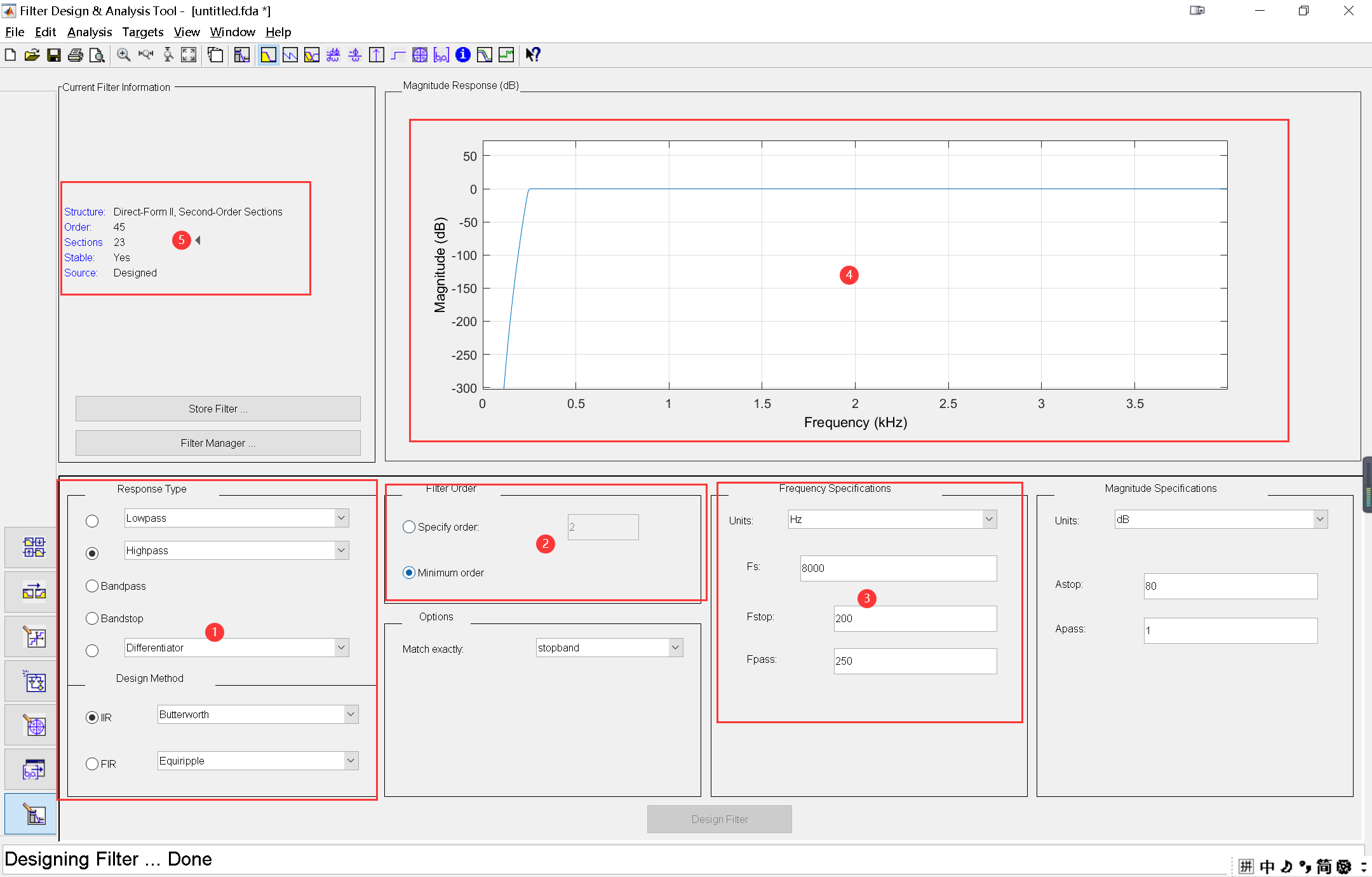
以下为对上图序号框区域的介绍：

1. 选择高通/低通/带通/带阻等滤波器类型以及滤波器实现方法（如IIR或FIR）；
2. 选择滤波器阶数，阶数越高，陡峭性越好；
3. 分别设置幅频特性坐标的单位，信号采样率，通带截止频率和阻带截止频率；
4. 该区域可以通过在Analysis菜单栏进行选择来显示该滤波器的不同参数指标或者数据分析；
5. 该区域为所设计滤波器的简要信息：结构，阶数，稳定性和滤波器来源。

②滤波器参数

  上图为我所设计的滤波器，为高通滤波器，IIR结构的巴特沃斯滤波器，阶数为由软件自动设置为符合条件的最小阶数45阶，原信号的采样率8000，通带截止频率为250Hz，阻带截止频率为200Hz。

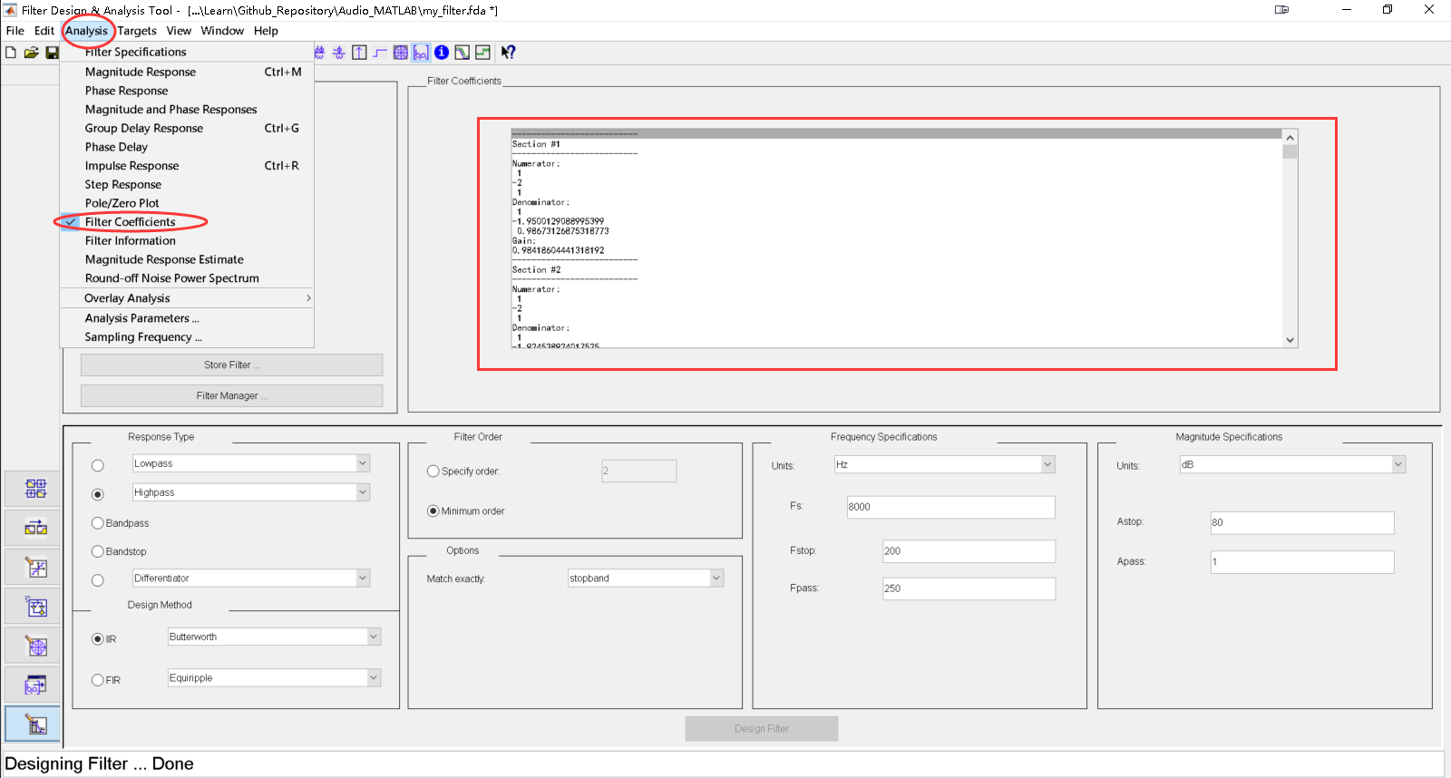
在上图所示的选项卡中可以看到滤波器系数，这个系数为系统函数H(Z)分子和分母在Z^（-n）前面的系数，它是由23个分式相乘而成。
  该工具生成的代码如下所示：

function Hd = my_filter_code2
%MY_FILTER_CODE2 Returns a discrete-time filter object.

% MATLAB Code
% Generated by MATLAB(R) 9.0 and the Signal Processing Toolbox 7.2.
% Generated on: 19-Oct-2022 14:56:51

% Butterworth Highpass filter designed using FDESIGN.HIGHPASS.

% All frequency values are in Hz.
Fs = 8000;  % Sampling Frequency

Fstop = 200; % Stopband Frequency
Fpass = 250; % Passband Frequency
Astop = 80;  % Stopband Attenuation (dB)
Apass = 1;   % Passband Ripple (dB)
match = 'stopband';  % Band to match exactly

% Construct an FDESIGN object and call its BUTTER method.
h  = fdesign.highpass(Fstop, Fpass, Astop, Apass, Fs);
Hd = design(h, 'butter', 'MatchExactly', match);

% [EOF]

3、利用该滤波器对混杂音频信号进行滤波

  主要代码如下：

% ==========MATLAB工具箱生成的滤波器========== %
H = my_filter_code2;
x_filtered = filter(H, x1);

x_filtered为已经被滤波的信号，H为所设计的滤波器。
滤波效果如下：

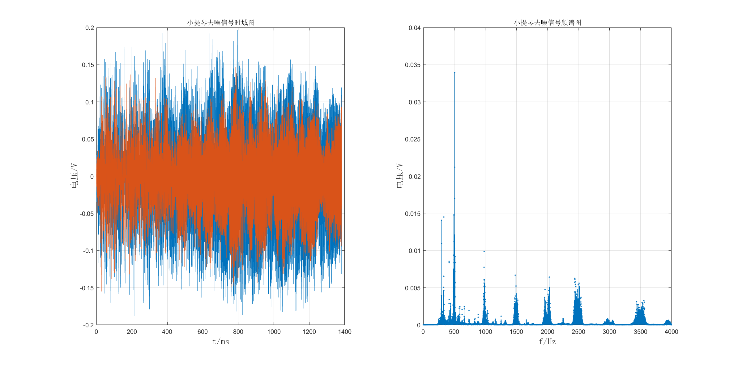
由图可见，低频部分的分量被很好滤除，且对比该图和原小提琴信号的时域和频域图，时域部分看不出差别，频域部分除被滤除的部分，其他部分基本一致。最后将滤波之后的数据用audiowrite函数导出得到.wav文件，其声音相对于混杂音频有极大的恢复且与原音频几乎没有差别。

附录：MATLAB代码

1、正弦信号处理代码

clear;
clc;
format long;
 
figure;
% ==========参数========== %
N = 10000;  % 整个图由N个样点构成
tscale = 6e-5;  % X轴显示的时间长度，单位为秒
dt = tscale / N;  % 每个样点间的时间间隔
t = 0 : dt : tscale;

f1 = 100000;  % 生成信号频率100kHz
f2 = 250000;  % 生成信号频率250kHz
f3 = 400000;  % 生成信号频率400kHz
A = 0.5;

% ==========生成正弦信号========== %
y1 = A * sin(2 * pi * f1 * t);  % 0.5为振幅。
y2 = A * sin(2 * pi * f2 * t);  % 0.5为振幅。
y3 = A * sin(2 * pi * f3 * t);  % 0.5为振幅。
 
% ==========画图========== %
subplot(3, 1, 1);
scatter(t .* 1000, y1, '.', 'k');  % 乘1000，将s换算成ms。
title('100kHz正弦信号');
axis([-inf, +inf, -1, +1]);  % 调节坐标显示范围。
xlabel('t/ms', 'FontName', '宋体', 'FontWeight', 'normal', 'FontSize', 14);
ylabel('电压/V', 'FontName', '宋体', 'FontWeight', 'normal', 'FontSize', 14);
grid on;

subplot(3, 1, 2);
scatter(t .* 1000, y2, '.', 'r');  % 乘1000，将s换算成ms。
title('250kHz正弦信号');
axis([-inf, +inf, -1, +1]);  % 调节坐标显示范围。
xlabel('t/ms', 'FontName', '宋体', 'FontWeight', 'normal', 'FontSize', 14);
ylabel('电压/V', 'FontName', '宋体', 'FontWeight', 'normal', 'FontSize', 14);
grid on;

subplot(3, 1, 3);
scatter(t .* 1000, y3, '.', 'b');  % 乘1000，将s换算成ms。
title('400kHz正弦信号');
axis([-inf, +inf, -1, +1]);  % 调节坐标显示范围。
xlabel('t/ms', 'FontName', '宋体', 'FontWeight', 'normal', 'FontSize', 14);
ylabel('电压/V', 'FontName', '宋体', 'FontWeight', 'normal', 'FontSize', 14);
grid on;

figure;
% ==========画采样后的图========== %
k = 1;
n_point = (k * tscale) / (1 / 500000);

t = linspace(0, k * tscale, n_point);
Y1 = A * sin(2 * pi * f1 * t);  % 0.5为振幅。
subplot(3, 2, 1);
stem(t .* 1000, Y1, '.');  % 乘1000，将s换算成ms。
title('500kHz采样信号');
axis([-inf, +inf, -1, +1]);  % 调节坐标显示范围。
xlabel('t/ms', 'FontName', '宋体', 'FontWeight', 'normal', 'FontSize', 14);
ylabel('电压/V', 'FontName', '宋体', 'FontWeight', 'normal', 'FontSize', 14);
grid on;

t = linspace(0, k * tscale, n_point);
Y2 = A * sin(2 * pi * f2 * t);  % 0.5为振幅。
subplot(3, 2, 3);
stem(t .* 1000, Y2, '.');  % 乘1000，将s换算成ms。
title('500kHz采样信号');
axis([-inf, +inf, -1, +1]);  % 调节坐标显示范围。
xlabel('t/ms', 'FontName', '宋体', 'FontWeight', 'normal', 'FontSize', 14);
ylabel('电压/V', 'FontName', '宋体', 'FontWeight', 'normal', 'FontSize', 14);
grid on;

t = linspace(0, k * tscale, n_point);
Y3 = A * sin(2 * pi * f3 * t);  % 0.5为振幅。
subplot(3, 2, 5);
stem(t .* 1000, Y3, '.');  % 乘1000，将s换算成ms。
title('500kHz采样信号');
axis([-inf, +inf, -1, +1]);  % 调节坐标显示范围。
xlabel('t/ms', 'FontName', '宋体', 'FontWeight', 'normal', 'FontSize', 14);
ylabel('电压/V', 'FontName', '宋体', 'FontWeight', 'normal', 'FontSize', 14);
grid on;

% ==========画采样后的频谱图========== %
fs = 500000;

yf1 = fft(Y1);
subplot(3, 2, 2);
realy = 2 * abs(yf1(1 : n_point)) / n_point;
realf = (0 : n_point - 1) * (fs / n_point);   
stem(realf, realy, '.');
title('100kHz正弦信号采样后频谱图');
axis([0, 500000, 0, 1]);
xlabel('f/Hz', 'FontName', '宋体', 'FontWeight', 'normal', 'FontSize', 14);
ylabel('电压/V', 'FontName', '宋体', 'FontWeight', 'normal', 'FontSize', 14);
grid on;

yf2 = fft(Y2);
subplot(3, 2, 4);
realy = 2 * abs(yf2(1 : n_point)) / n_point;  % 频率为250kHz时幅度大于0.5V。
realf = (0 : n_point - 1) * (fs / n_point);  
stem(realf, realy, '.');
title('250kHz正弦信号采样后频谱图');
axis([0, 500000, 0, 1]);
xlabel('f/Hz', 'FontName', '宋体', 'FontWeight', 'normal', 'FontSize', 14);
ylabel('电压/V', 'FontName', '宋体', 'FontWeight', 'normal', 'FontSize', 14);
grid on;

yf3 = fft(Y3);
subplot(3, 2, 6);
realy = 2 * abs(yf3(1 : n_point)) / n_point;
realf = (0 : n_point - 1) * (fs / n_point);  
stem(realf, realy, '.');
title('500kHz正弦信号采样后频谱图');
axis([0, 500000, 0, 1]);
xlabel('f/Hz', 'FontName', '宋体', 'FontWeight', 'normal', 'FontSize', 14);
ylabel('电压/V', 'FontName', '宋体', 'FontWeight', 'normal', 'FontSize', 14);
grid on;

% ==========恢复波形========== %
%原理(内插法): y(t)=Σx(n)*sinc((t-nTs)/Ts)
n_point = (k * tscale) / (1 / 500000);  % 采样点数
ts = 1 / fs;  % 采样时间间隔
to = linspace(0, k * tscale, n_point);
K = 30;  % 还原后的信号点倍数
dt = ts / K;  % 还原后的点时间间隔
ta = 0 : dt : n_point * ts;

figure;
% =====信号1===== %
y_recover1 = zeros(length(ta), 1);  % 恢复信号y，先建立一个0矩阵，从0到1，时间间隔为dt
for t = 0 : length(ta) - 1  % 求过采样后的每个值
	for m = 0 : length(to) - 1  % 累加sinc与原函数对应点的积
		y_recover1(t + 1) = y_recover1(t + 1) + Y1(m + 1) * sinc((t * dt - m * ts) / ts);
	end
end

subplot(3, 1, 1);
scatter(ta.* 1000, y_recover1, '.');
title('100kHz重建信号(内插法)');
axis([-inf, +inf, -1, +1]);  % 调节坐标显示范围。
xlabel('t/ms', 'FontName', '宋体', 'FontWeight', 'normal', 'FontSize', 14);
ylabel('电压/V', 'FontName', '宋体', 'FontWeight', 'normal', 'FontSize', 14);
grid on;

% =====信号2===== %
y_recover2 = zeros(length(ta), 1);  % 恢复信号y，先建立一个0矩阵，从0到1，时间间隔为dt
for t = 0 : length(ta) - 1  % 求过采样后的每个值
	for m = 0 : length(to) - 1  % 累加sinc与原函数对应点的积
		y_recover2(t + 1) = y_recover2(t + 1) + Y2(m + 1) * sinc((t * dt - m * ts) / ts);
	end
end

subplot(3, 1, 2);
scatter(ta.* 1000, y_recover2, '.');
title('250kHz重建信号(内插法)');
axis([-inf, +inf, -1, +1]);  % 调节坐标显示范围。
xlabel('t/ms', 'FontName', '宋体', 'FontWeight', 'normal', 'FontSize', 14);
ylabel('电压/V', 'FontName', '宋体', 'FontWeight', 'normal', 'FontSize', 14);
grid on;

% =====信号3===== %
y_recover3 = zeros(length(ta), 1);  % 恢复信号y，先建立一个0矩阵，从0到1，时间间隔为dt
for t = 0 : length(ta) - 1  % 求过采样后的每个值
	for m = 0 : length(to) - 1  % 累加sinc与原函数对应点的积
		y_recover3(t + 1) = y_recover3(t + 1) + Y3(m + 1) * sinc((t * dt - m * ts) / ts);
	end
end

subplot(3, 1, 3);
scatter(ta.* 1000, y_recover3, '.');
title('500kHz重建信号(内插法)');
axis([-inf, +inf, -1, +1]);  % 调节坐标显示范围。
xlabel('t/ms', 'FontName', '宋体', 'FontWeight', 'normal', 'FontSize', 14);
ylabel('电压/V', 'FontName', '宋体', 'FontWeight', 'normal', 'FontSize', 14);
grid on;

2、语音信号处理代码

clear;
clc;
format long;

figure;
% ==========原始信号========== %
[x, fs] = audioread('./武汉.wav');

N = 14000;  % 整个图由N个样点构成
dt = 1 / fs;
tscale = dt * N;  % X轴显示的时间长度，单位为秒
t = 0 : dt : tscale - tscale / N;

subplot(1, 2, 1);
plot(t .* 1000, x);
title('原语音信号时域图');
xlabel('t/ms', 'FontName', '宋体', 'FontWeight', 'normal', 'FontSize', 14);
ylabel('电压/V', 'FontName', '宋体', 'FontWeight', 'normal', 'FontSize', 14);
grid on;

y = fft(x);
realy = 2 * abs(y(1 : length(x))) / length(x);
realf = (0 : length(x) - 1) * (fs / length(x)); 
subplot(1, 2, 2);
stem(realf, realy, '.');
title('原语音信号频谱图');
axis([0, 1000, 0, 0.04]);
xlabel('f/Hz', 'FontName', '宋体', 'FontWeight', 'normal', 'FontSize', 14);
ylabel('电压/V', 'FontName', '宋体', 'FontWeight', 'normal', 'FontSize', 14);
grid on;

figure;
% ==========减少采样率后的信号========== %
% 人的语音信号频率在0到600Hz之间，从原信号频谱可以看出信号能量在100到500Hz之间，因此以下取采样率为2000Hz为过采样，1000Hz为临界采样，800Hz为欠采样。
% =====过采样===== %
x1 = decimate(x, 4);
t1 = decimate(t, 4);
fs1 = fs / 4;
subplot(3, 2, 1);
plot(t1 .* 1000, x1);
title('过采样语音信号时域图');
xlabel('t/ms', 'FontName', '宋体', 'FontWeight', 'normal', 'FontSize', 14);
ylabel('电压/V', 'FontName', '宋体', 'FontWeight', 'normal', 'FontSize', 14);
grid on;

y1 = fft(x1);
realy = 2 * abs(y1(1 : length(x1))) / length(x1);
realf = (0 : length(x1) - 1) * (fs1 / length(x1)); 
subplot(3, 2, 2);
stem(realf, realy, '.');
title('过采样语音信号频谱图');
axis([0, 2000, 0, 0.04]);
xlabel('f/Hz', 'FontName', '宋体', 'FontWeight', 'normal', 'FontSize', 14);
ylabel('电压/V', 'FontName', '宋体', 'FontWeight', 'normal', 'FontSize', 14);
grid on;

% =====临界采样===== %
x2 = decimate(x, 8);
t2 = decimate(t, 8);
fs2 = fs / 8;
subplot(3, 2, 3);
plot(t2 .* 1000, x2);
title('临界采样语音信号时域图');
xlabel('t/ms', 'FontName', '宋体', 'FontWeight', 'normal', 'FontSize', 14);
ylabel('电压/V', 'FontName', '宋体', 'FontWeight', 'normal', 'FontSize', 14);
grid on;

y2 = fft(x2);
realy = 2 * abs(y2(1 : length(x2))) / length(x2);
realf = (0 : length(x2) - 1) * (fs2 / length(x2)); 
subplot(3, 2, 4);
stem(realf, realy, '.');
title('临界采样语音信号频谱图');
axis([0, 1000, 0, 0.04]);
xlabel('f/Hz', 'FontName', '宋体', 'FontWeight', 'normal', 'FontSize', 14);
ylabel('电压/V', 'FontName', '宋体', 'FontWeight', 'normal', 'FontSize', 14);
grid on;

% =====欠采样===== %
x3 = decimate(x, 10);
t3 = decimate(t, 10);
fs3 = fs / 10;
subplot(3, 2, 5);
plot(t3 .* 1000, x3);
title('欠采样语音信号时域图');
xlabel('t/ms', 'FontName', '宋体', 'FontWeight', 'normal', 'FontSize', 14);
ylabel('电压/V', 'FontName', '宋体', 'FontWeight', 'normal', 'FontSize', 14);
grid on;

y3 = fft(x3);
realy = 2 * abs(y3(1 : length(x3))) / length(x3);
realf = (0 : length(x3) - 1) * (fs3 / length(x3)); 
subplot(3, 2, 6);
stem(realf, realy, '.');
title('欠采样语音信号频谱图');
axis([0, 800, 0, 0.04]);
xlabel('f/Hz', 'FontName', '宋体', 'FontWeight', 'normal', 'FontSize', 14);
ylabel('电压/V', 'FontName', '宋体', 'FontWeight', 'normal', 'FontSize', 14);
grid on;

figure;
% ==========减少采样率后的信号恢复========== %
f = 8000;
f1 = 2000;
f2 = 1000;
f3 = 800;
tscale = 1;

% =====过采样===== %
n_point = 14000 / 4;  % 采样点数
ts = 1 / f1;  % 采样时间间隔
to = linspace(0, tscale, n_point);
K = 4;  % 还原后的信号点倍数
dt = ts / K;  % 还原后的点时间间隔
ta = 0 : dt : n_point * ts;
y_recover1 = zeros(length(ta), 1);  % 恢复信号y，先建立一个0矩阵，从0到1，时间间隔为dt

for t = 0 : length(ta) - 1  % 求过采样后的每个值
	for m = 0 : length(to) - 1  % 累加sinc与原函数对应点的积
		y_recover1(t + 1) = y_recover1(t + 1) + x1(m + 1) * sinc((t * dt - m * ts) / ts);
	end
end

subplot(3, 2, 1);
plot(ta.* 1000, y_recover1);
title('过采样重建信号(内插法)');
axis([-inf, +inf, -1, +1]);  % 调节坐标显示范围。
xlabel('t/ms', 'FontName', '宋体', 'FontWeight', 'normal', 'FontSize', 14);
ylabel('电压/V', 'FontName', '宋体', 'FontWeight', 'normal', 'FontSize', 14);
grid on;

Y1 = fft(y_recover1);
realy = 2 * abs(Y1(1 : length(y_recover1))) / length(y_recover1);
realf = (0 : length(y_recover1) - 1) * (fs / length(y_recover1)); 
subplot(3, 2, 2);
stem(realf, realy, '.');
title('过采样语音信号恢复后频谱图');
axis([0, 1000, 0, 0.04]);
xlabel('f/Hz', 'FontName', '宋体', 'FontWeight', 'normal', 'FontSize', 14);
ylabel('电压/V', 'FontName', '宋体', 'FontWeight', 'normal', 'FontSize', 14);
grid on;

% =====临界采样===== %
n_point = 14000 / 8;  % 采样点数
ts = 1 / f2;  % 采样时间间隔
to = linspace(0, tscale, n_point);
K = 8;  % 还原后的信号点倍数
dt = ts / K;  % 还原后的点时间间隔
ta = 0 : dt : n_point * ts;
y_recover2 = zeros(length(ta), 1);  % 恢复信号y，先建立一个0矩阵，从0到1，时间间隔为dt

for t = 0 : length(ta) - 1  % 求过采样后的每个值
	for m = 0 : length(to) - 1  % 累加sinc与原函数对应点的积
		y_recover2(t + 1) = y_recover2(t + 1) + x2(m + 1) * sinc((t * dt - m * ts) / ts);
	end
end

subplot(3, 2, 3);
plot(ta.* 1000, y_recover2);
title('临界采样重建信号(内插法)');
axis([-inf, +inf, -1, +1]);  % 调节坐标显示范围。
xlabel('t/ms', 'FontName', '宋体', 'FontWeight', 'normal', 'FontSize', 14);
ylabel('电压/V', 'FontName', '宋体', 'FontWeight', 'normal', 'FontSize', 14);
grid on;

Y2 = fft(y_recover2);
realy = 2 * abs(Y2(1 : length(y_recover2))) / length(y_recover2);
realf = (0 : length(y_recover2) - 1) * (fs / length(y_recover2)); 
subplot(3, 2, 4);
stem(realf, realy, '.');
title('临界采样语音信号恢复后频谱图');
axis([0, 1000, 0, 0.04]);
xlabel('f/Hz', 'FontName', '宋体', 'FontWeight', 'normal', 'FontSize', 14);
ylabel('电压/V', 'FontName', '宋体', 'FontWeight', 'normal', 'FontSize', 14);
grid on;

% =====欠采样===== %
n_point = 14000 / 10;  % 采样点数
ts = 1 / f3;  % 采样时间间隔
to = linspace(0, tscale, n_point);
K = 10;  % 还原后的信号点倍数
dt = ts / K;  % 还原后的点时间间隔
ta = 0 : dt : n_point * ts;
y_recover3 = zeros(length(ta), 1);  % 恢复信号y，先建立一个0矩阵，从0到1，时间间隔为dt

for t = 0 : length(ta) - 1  % 求过采样后的每个值
	for m = 0 : length(to) - 1  % 累加sinc与原函数对应点的积
		y_recover3(t + 1) = y_recover3(t + 1) + x3(m + 1) * sinc((t * dt - m * ts) / ts);
	end
end

subplot(3, 2, 5);
plot(ta.* 1000, y_recover3);
title('欠采样重建信号(内插法)');
axis([-inf, +inf, -1, +1]);  % 调节坐标显示范围。
xlabel('t/ms', 'FontName', '宋体', 'FontWeight', 'normal', 'FontSize', 14);
ylabel('电压/V', 'FontName', '宋体', 'FontWeight', 'normal', 'FontSize', 14);
grid on;

Y2 = fft(y_recover2);
realy = 2 * abs(Y2(1 : length(y_recover2))) / length(y_recover2);
realf = (0 : length(y_recover2) - 1) * (fs / length(y_recover2)); 
subplot(3, 2, 6);
stem(realf, realy, '.');
title('临界采样语音信号恢复后频谱图');
axis([0, 1000, 0, 0.04]);
xlabel('f/Hz', 'FontName', '宋体', 'FontWeight', 'normal', 'FontSize', 14);
ylabel('电压/V', 'FontName', '宋体', 'FontWeight', 'normal', 'FontSize', 14);
grid on;

3、小提琴音频的加噪去噪处理代码

clear;
clc;
format long;

% ==========原始信号========== %
[x1, fs1] = audioread('./Audio/小提琴.wav');

N1 = length(x1);  % 整个图由N1个样点构成
dt1 = 1 / fs1;
tscale1 = dt1 * N1;  % X轴显示的时间长度，单位为秒
t1 = 0 : dt1 : tscale1 - tscale1 / N1;

subplot(1, 2, 1);
plot(t1 .* 1000, x1);
title('小提琴信号时域图');
xlabel('t/ms', 'FontName', '宋体', 'FontWeight', 'normal', 'FontSize', 14);
ylabel('电压/V', 'FontName', '宋体', 'FontWeight', 'normal', 'FontSize', 14);
grid on;

y1 = fft(x1);
realy = 2 * abs(y1(1 : length(x1))) / length(x1);
realf = (0 : length(x1) - 1) * (fs1 / length(x1)); 
subplot(1, 2, 2);
stem(realf, realy, '.');
title('小提琴信号频谱图');
axis([0, 4000, 0, 0.04]);
xlabel('f/Hz', 'FontName', '宋体', 'FontWeight', 'normal', 'FontSize', 14);
ylabel('电压/V', 'FontName', '宋体', 'FontWeight', 'normal', 'FontSize', 14);
grid on;

figure;
% ==========噪声信号========== %
[x3, fs3] = audioread('./Audio/噪声.wav');

N3 = length(x3);  % 整个图由N1个样点构成
dt3 = 1 / fs3;
tscale3 = dt3 * N3;  % X轴显示的时间长度，单位为秒
t3 = 0 : dt3 : tscale3 - tscale3 / N3;

subplot(1, 2, 1);
plot(t3 .* 1000, x3);
title('小提琴信号时域图');
xlabel('t/ms', 'FontName', '宋体', 'FontWeight', 'normal', 'FontSize', 14);
ylabel('电压/V', 'FontName', '宋体', 'FontWeight', 'normal', 'FontSize', 14);
grid on;

y3 = fft(x3);
realy = 2 * abs(y3(1 : length(x3))) / length(x3);
realf = (0 : length(x3) - 1) * (fs3 / length(x3)); 
subplot(1, 2, 2);
stem(realf, realy, '.');
title('小提琴信号频谱图');
axis([0, 4000, 0, 0.04]);
xlabel('f/Hz', 'FontName', '宋体', 'FontWeight', 'normal', 'FontSize', 14);
ylabel('电压/V', 'FontName', '宋体', 'FontWeight', 'normal', 'FontSize', 14);
grid on;

figure;
% -------------------- %
[x2, fs2] = audioread('./Audio/小提琴混杂声音_缩混.wav');

N2 = length(x2);  % 整个图由N2个样点构成
dt2 = 1 / fs2;
tscale2 = dt2 * N2;  % X轴显示的时间长度，单位为秒
t2 = 0 : dt2 : tscale2 - tscale2 / N2;

subplot(1, 2, 1);
plot(t2 .* 1000, x2);
title('小提琴混杂噪声信号时域图');
xlabel('t/ms', 'FontName', '宋体', 'FontWeight', 'normal', 'FontSize', 14);
ylabel('电压/V', 'FontName', '宋体', 'FontWeight', 'normal', 'FontSize', 14);
grid on;

y2 = fft(x2);
realy = 2 * abs(y2(1 : length(x2))) / length(x2);
realf = (0 : length(x2) - 1) * (fs2 / length(x2)); 
subplot(1, 2, 2);
stem(realf, realy, '.');
title('小提琴混杂噪声信号频谱图');
axis([0, 4000, 0, 0.04]);
xlabel('f/Hz', 'FontName', '宋体', 'FontWeight', 'normal', 'FontSize', 14);
ylabel('电压/V', 'FontName', '宋体', 'FontWeight', 'normal', 'FontSize', 14);
grid on;

figure;
% ==========MATLAB工具箱生成的滤波器========== %
H = my_filter_code2;
x_filtered = filter(H, x1);

subplot(1, 2, 1);
plot(t1 .* 1000, x_filtered);
title('小提琴去噪信号时域图');
xlabel('t/ms', 'FontName', '宋体', 'FontWeight', 'normal', 'FontSize', 14);
ylabel('电压/V', 'FontName', '宋体', 'FontWeight', 'normal', 'FontSize', 14);
grid on;

y_filtered = fft(x_filtered);
realy = 2 * abs(y_filtered(1 : length(x_filtered))) / length(x_filtered);
realf = (0 : length(x_filtered) - 1) * (fs2 / length(x_filtered)); 
subplot(1, 2, 2);
stem(realf, realy, '.');
title('小提琴去噪信号频谱图');
axis([0, 4000, 0, 0.04]);
xlabel('f/Hz', 'FontName', '宋体', 'FontWeight', 'normal', 'FontSize', 14);
ylabel('电压/V', 'FontName', '宋体', 'FontWeight', 'normal', 'FontSize', 14);
grid on;

audiowrite('./Audio/小提琴去噪.wav', x_filtered, 8000);

转载自CSDN-专业IT技术社区

版权声明：本文为博主原创文章，遵循 CC 4.0 BY-SA 版权协议，转载请附上原文出处链接和本声明。

原文链接：https://blog.csdn.net/SnowyForest___/article/details/127423981