
引言:
在分子动力学(MD)模拟的后处理中,沿某个方向的空间分布(profile)是非常常见的分析需求,例如数密度/质量密度、速度分布、应力(压力)分布、电荷分布、势能分布等。理想情况下,我们可以在 LAMMPS 的
in文件里用compute chunk/atom+fix ave/chunk在运行过程中直接对空间分箱(binning)并做时间平均;而且fix ave/chunk还能对多种 per-atom 量(如速度、力、电荷、势能、应力等)做按 chunk 的汇总/平均输出。但很多时候模拟已经跑完,脚本里没写这些 profile 计算,手头只剩下轨迹文件(dump/xyz/lammpstrj)。这时再回去重跑既费时又不必要——更合适的做法是:使用 后处理工具从轨迹中重新统计分布。
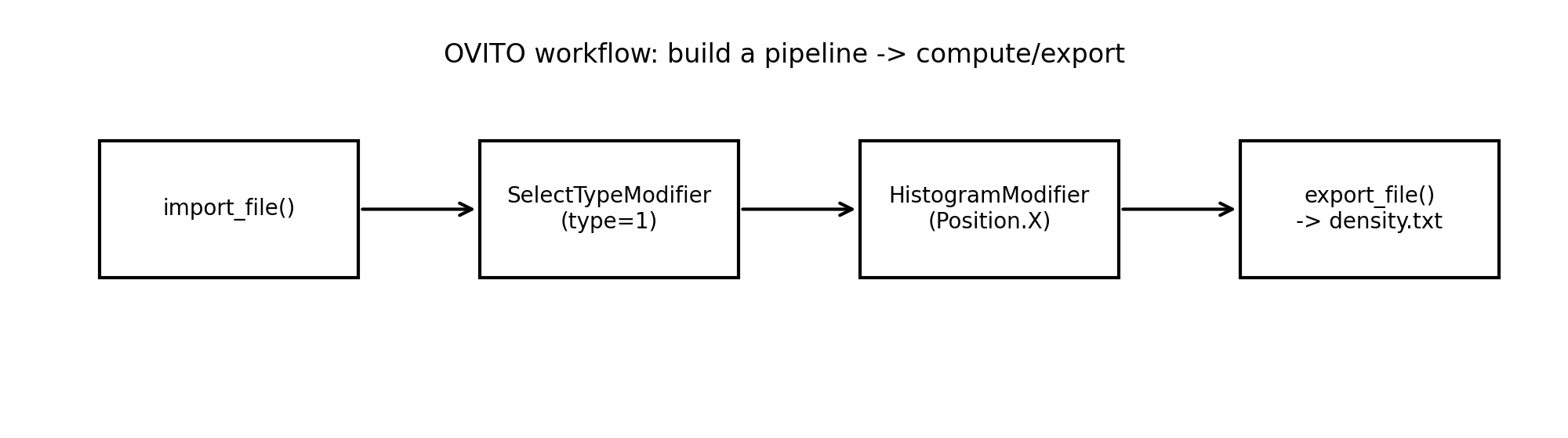
OVITO 的 Python 模块提供了一套非常清晰的“数据流水线(pipeline)”机制:导入数据(
import_file)→ 依次应用 modifiers →compute()得到结果 →export_file导出,非常适合把后处理流程脚本化、自动化。
一、 为什么要做“后处理密度分布”
在 LAMMPS 里,密度/电荷/速度/应力等空间分布,本来可以在 in 文件里通过 chunk + 平均直接算出来(典型做法是 compute chunk/atom + fix ave/chunk),并输出为 profile 文件。LAMMPS 官方文档也明确:chunks 可以按空间 bin 切分,并对每个 chunk 统计包括密度、速度、应力、势能等多种量。
但现实经常是:
计算已经跑完了;
当时没有在
in文件里写 profile 的计算;现在只剩 dump/xyz 轨迹文件。
这时就需要后处理。OVITO 的 Python 模块非常适合做这一类“按空间分箱统计”的任务:读取轨迹 → 选择原子子集 → 做直方图/分箱 → 导出表格。
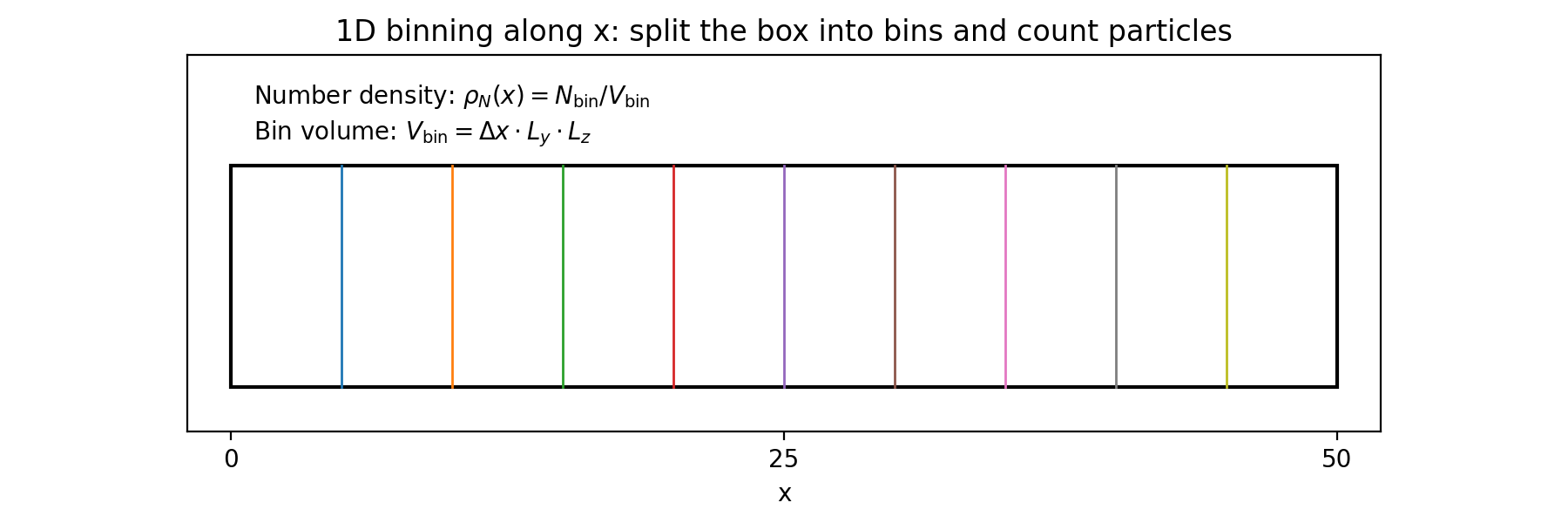
二、核心原理:直方图(Histogram)= 沿 x 方向分箱计数
我们把盒子在 x 方向切成 bin_count 个小区间(bin),对每个 bin:
-
计数:NbinN_{\text{bin}}Nbin(这个 bin 里有多少个目标原子)
-
若要“数密度”(number density)而不仅是计数:

其中 Ly,LzL_y,L_zLy,Lz 是盒子在 y,z 方向长度(假设截面积不随时间变化或你逐帧计算)。
OVITO 的 HistogramModifier 支持多种归一化方式:
-
AbsoluteCount(每个 bin 的样本数) -
RelativeFrequency(频率 = bin_count / 总样本数) -
ProbabilityDensity(概率密度 = bin_count / 总样本数 / bin_width)
这些模式在 OVITO 3.13.0 起提供。
注意:
ProbabilityDensity是“概率密度”,不是物理意义上的“数密度(#/体积)”。要得到真正数密度,仍建议用 VbinV_{\text{bin}}Vbin 做体积归一化。
三、环境准备:安装 OVITO Python 模块
两种常见方式:
方式 A:pip(普通 Python 环境)
PyPI 页面列出了支持的平台与 Python 版本范围(例如 Windows/Linux x86_64、Python 3.10–3.13 等)。
方式 B:conda(推荐给 conda 用户)
OVITO 官方给了 conda 安装命令(含 ovito 模块;并提示 conda 包也可能带桌面端组件)。
四、数据准备:你能统计什么,取决于 dump 里有什么
4.1 统计密度(位置分布)最低要求
dump/xyz 至少要有:
-
Particle Type(或 type) -
Position.X/Y/Z
如果你用的是legacy XYZ(列含义不固定),需要用 import_file(..., columns=[...]) 显式告诉 OVITO 每一列是什么含义,例如:
pipeline = import_file(
    "dump.xyz",
    columns=["Particle Type", "Position.X", "Position.Y", "Position.Z"]
)
OVITO 的 import_file() 会自动识别格式并创建 pipeline。
4.2 想统计速度/势能/应力:必须提前写进 dump
-
速度:dump 里要有
vx vy vz -
势能:需要 LAMMPS
compute pe/atom并dump custom输出该列。 -
应力:需要
compute stress/atom(或相关命令)并输出到 dump;LAMMPS 文档也给过“用 per-atom stress 做 1D 压力 profile”的示例思路。
关键提醒:后处理不能凭空“算出”你没输出的 per-atom 势能/应力。OVITO 能做的是:对“文件里已有的每原子属性”进行统计、分箱、平均。
五、最小可用:Type=1 原子沿 x 的直方图(你给的代码增强版)
你原始代码非常接近正确,但建议补上两点:
from ovito.modifiers import HistogramModifier, SelectTypeModifier
from ovito.io import import_file, export_file

pipeline = import_file("dump.xyz")  # 或 dump.lammpstrj 等

# 选出 Type=1
pipeline.modifiers.append(
    SelectTypeModifier(operate_on="particles", property="Particle Type", types={1})
)

# 沿 x 分箱做直方图
hist = HistogramModifier(
    operate_on="particles",
    property="Position.X",
    bin_count=15,
    only_selected=True,
)
hist.fix_xrange = True
hist.xrange_start = 0
hist.xrange_end = 50

# 绝对计数(默认就是这个)
hist.normalization = HistogramModifier.NormalizationMode.AbsoluteCount

pipeline.modifiers.append(hist)

# HistogramModifier 会生成一个 DataTable,名字通常类似 histogram[Position.X]
export_file(pipeline, "density.txt", "txt/table", key="histogram[Position.X]")
-
SelectTypeModifier的用法:按某个 property(例如 Particle Type)选择指定类型。 -
HistogramModifier的关键参数:property、bin_count、only_selected、fix_xrange/xrange_start/xrange_end、normalization。
“key=...到底是什么?”
很多 modifier 会把结果以 DataTable 的形式放进 pipeline 输出里,然后 export_file(..., key=...) 指定导出哪张表。OVITO 文档示例明确展示了这种模式(比如导出 key='binning' 的表)。
实战建议:你可以先打印一下有哪些表:
data = pipeline.compute()
print(list(data.tables.keys()))
然后把 key 改成你实际看到的名字。
六、真正的“数密度”怎么做(把计数除以体积)
上面的 density.txt 本质是“每个 bin 的计数”。要变成数密度(#/体积),你需要盒子尺寸 Ly,LzL_y,L_zLy,Lz(以及 bin 宽度 Δx\Delta xΔx)。
下面给一个新手友好的脚本:导出两列:bin_center 与 number_density
import numpy as np
from ovito.modifiers import HistogramModifier, SelectTypeModifier
from ovito.io import import_file

pipeline = import_file("dump.xyz")
pipeline.modifiers.append(SelectTypeModifier(property="Particle Type", types={1}))

hist = HistogramModifier(property="Position.X", bin_count=15, only_selected=True)
hist.fix_xrange = True
hist.xrange_start = 0
hist.xrange_end = 50
hist.normalization = HistogramModifier.NormalizationMode.AbsoluteCount
pipeline.modifiers.append(hist)

data = pipeline.compute()

# 取出 histogram 表
table = data.tables["histogram[Position.X]"]

# 不同版本表列名可能略不同,最稳妥是打印 table.columns
# print(table.columns)

# 这里用“通用思路”:第一列通常是 bin center,第二列是 count
bin_center = np.array(table[:, 0])
count = np.array(table[:, 1])

# 盒子尺寸:data.cell 是模拟盒信息(假设正交盒)
# 若是三斜晶胞,需要更谨慎地取横截面积(这里先给初学者版)
Ly = data.cell[:, 1].length
Lz = data.cell[:, 2].length
dx = (hist.xrange_end - hist.xrange_start) / hist.bin_count
Vbin = dx * Ly * Lz

number_density = count / Vbin

np.savetxt(
    "number_density_x.txt",
    np.column_stack([bin_center, number_density]),
    header="bin_center  number_density(#/volume)",
    comments=""
)
如果你是 NPT、盒子会变化:建议逐帧计算并平均(下一节给模板)。
七、 进阶:轨迹多帧平均(更接近论文里的“平均密度剖面”)
OVITO 的轨迹是“按需加载”的:不会一次读入所有帧,而是你
compute(frame)时读那一帧。
因此你可以这样做“逐帧累加 + 平均”:
import numpy as np
from ovito.io import import_file
from ovito.modifiers import SelectTypeModifier, HistogramModifier

pipeline = import_file("dump.xyz")
pipeline.modifiers.append(SelectTypeModifier(property="Particle Type", types={1}))

hist = HistogramModifier(property="Position.X", bin_count=100, only_selected=True)
hist.fix_xrange = True
hist.xrange_start = 0
hist.xrange_end = 50
pipeline.modifiers.append(hist)

sum_count = None
bin_center = None
nframes = pipeline.num_frames

for frame in range(nframes):
    data = pipeline.compute(frame)
    table = data.tables["histogram[Position.X]"]
    bc = np.array(table[:, 0])
    ct = np.array(table[:, 1])

    if sum_count is None:
        sum_count = ct.copy()
        bin_center = bc
    else:
        sum_count += ct

avg_count = sum_count / nframes
np.savetxt("avg_count_x.txt", np.column_stack([bin_center, avg_count]),
           header="bin_center  avg_count", comments="")
八、 常见坑(新手必看)
-
XYZ 列映射没写:legacy XYZ 必须用
columns=[...]指定列含义,否则 OVITO 不知道哪列是 type、哪列是 x/y/z。 -
设置了 xrange_start/end 但没生效:要
fix_xrange=True。 -
把“计数”当成“密度”:真正数密度要除以 bin 体积(或至少除以 bin 宽度做 1D 线密度)。
-
想统计势能/应力但 dump 没有:后处理救不了;只能回到 LAMMPS 增加输出(如
compute pe/atom、compute stress/atom)再跑或重 dump。 -
Key 写错:先
print(data.tables.keys())看看实际表名,再填export_file(..., key=...)。OVITO 文档给过这种“按 key 导出表”的范式示例。
九、与我联系——交流疑问
了解清楚了安装之前的这些知识以后,如果嫌弃麻烦需要远程安装的友友可以联系!
PC端电脑通过
点击PC端分子对接软件合集——“能看到某宝对应的分子对接软件商品!!!。
手机淘宝通过:
点击手淘分子对接软件合集 “——能看到某宝对应的分子对接软件商品!!!
转载自CSDN-专业IT技术社区
原文链接:https://blog.csdn.net/GHZ2443063059/article/details/156192197